| .vscode | ||
| documentation | ||
| examples | ||
| readme_media | ||
| src | ||
| README.md | ||
Purpose
This repository is designed to model, simulate, and analyze systems that incorporate sensor networks for physical measurements. Using Monte Carlo simulations, the system evaluates the uncertainty and sensitivity of various sensors and provides detailed insights into how errors propagate in multi-sensor setups. This tool is especially useful for engineers and scientists involved in instrumentation, metrology, and process analysis.
Monte-Carlo Simulation Setup
The Monte Carlo simulation framework in this repository allows users to:
- Define sensor networks, including their error characteristics.
- Combine multiple sensors to calculate derived quantities (e.g., mass flow rate).
- Perform sensitivity and range analyses to evaluate the impact of individual sensor errors on system performance.
- Generate reports summarizing system uncertainty and sensitivity results.
To set up and run the simulation:
-
Wherever your working directory is, copy src/System_Uncertainty_Monte_Carlo.py and src/PDF_Generator into your working directory.
-
Copy the folder code/inputs into your working directory.
-
Create a new python file for your project.
-
Import the header boilerplate
import matplotlib.pyplot as plt
import math

from inputs.Inputs import AveragingInput, PhysicalInput
from inputs.Pressure_Sensors import PressureTransmitter
from inputs.Temperature_Sensors import RTD, Thermocouple
from inputs.Force_Sensors import LoadCell
from inputs.Flow_Speed_Sensors import TurbineFlowMeter
from inputs.Fluid_Lookup import DensityLookup
from inputs.Math_Functions import Integration

from System_Uncertainty_Monte_Carlo import SystemUncertaintyMonteCarlo
-
Create your sensors and final output expression and run the simulation.
-
Output files will be put in your "working directory/Output Files/"
Types of Sensors
The repository supports various sensor types, including:
- Pressure Sensors (e.g., Pressure Transmitters)
- Temperature Sensors (e.g., RTDs and Thermocouples)
- Flow Speed Sensors (e.g., Turbine Flow Meters)
- Physical Property Sensors (e.g., Pipe Diameter Measurements)
- Combined Inputs (e.g., density lookup derived from pressure and temperature sensors)
Each sensor type can have its own error characteristics, such as repeatability, hysteresis, non-linearity, and temperature-induced offsets, which are considered in the uncertainty analysis.
Examples
Mass Flow Rate Through Pipe
The example in examples/mass_flow_rate.py demonstrates how to estimate the mass flow rate through a pipe using a network of sensors. The system consists of:
- Two Pressure Transmitters: Averaged using the
AveragingInputclass to estimate the mean pressure. - One RTD: Used to measure temperature and assist in density calculations.
- One Turbine Flow Meter: Measures flow speed.
Key Code Snippets
Pre-Defining Sensor Errors
# Define true values and sensor error ranges
pt_1_errors = {
    "k": 2,                             # How many standard deviations each of these errors represents (if applicable)
    "fso": 100,                         # full scale output so that stdev can be calculated for errors based on FSO
    "static_error_band": 0.15,          # +-% of FSO
    "repeatability": 0.02,              # +-% of FSO
    "hysteresis": 0.07,                 # +-% of FSO
    "non-linearity": 0.15,              # +-% of FSO
    "temperature_zero_error": 0.005,    # +% of FSO per degree F off from calibration temp
    "temperature_offset": 30,           # Degrees F off from calibration temp
}

RTD_1_errors = {
    "k": 3,                             # How many standard deviations each of these errors represents (if applicable)
     "class": "A",                      # class AA, A, B, C
}

flow_1_errors = {
    "k": 2,                             # How many standard deviations each of these errors represents (if applicable)
    "fso": 20,                          # full scale output so that stdev can be calculated for errors based on FSO
    "static_error_band": 0.25,          # +-% of FSO
}

pipe_diameter_error = {
    "tolerance": 0.05,
    "cte": 8.8E-6,                       # degrees F^-1
    "temperature_offset": -100           # Degrees off from when the measurement was taken
}
Defining Sensors
# Create sensor instances
pressure_transmitter_1 = PressureTransmitter(25, pt_1_errors, name="PT 1")
pressure_transmitter_2 = PressureTransmitter(20, pt_1_errors, name="PT 2")
temperature_sensor_1 = RTD(250, RTD_1_errors, name="RTD 1")
flow_speed = TurbineFlowMeter(10, flow_1_errors, "Flow Sensor 1")

# Physical property
pipe_diameter = PhysicalInput(1, pipe_diameter_error, name="Pipe Diameter")
Combining Inputs for Derived Properties
# Combining the two pressure sensors for an averaged value. Can be done with AveragingInput or mathematically
average_pressure = AveragingInput([pressure_transmitter_1, pressure_transmitter_2])

# Create DensityLookup instance
density_lookup = DensityLookup(pressure_sensor=average_pressure, temperature_sensor=temperature_sensor_1)

# Define the combined sensor
combined_input = math.pi * density_lookup * flow_speed * (pipe_diameter / 12 / 2)**2
Running Monte Carlo Analysis
monte_carlo = SystemUncertaintyMonteCarlo(combined_input)
monte_carlo.perform_system_analysis({
    "num_runs": 1000,
    "num_processes": 10
})
monte_carlo.save_report()
This example illustrates the process of setting up sensors, combining their outputs into derived quantities, and performing a detailed uncertainty analysis using Monte Carlo simulations.
PDF Report
The PDF report associated with the mass flow rate example can be found here.
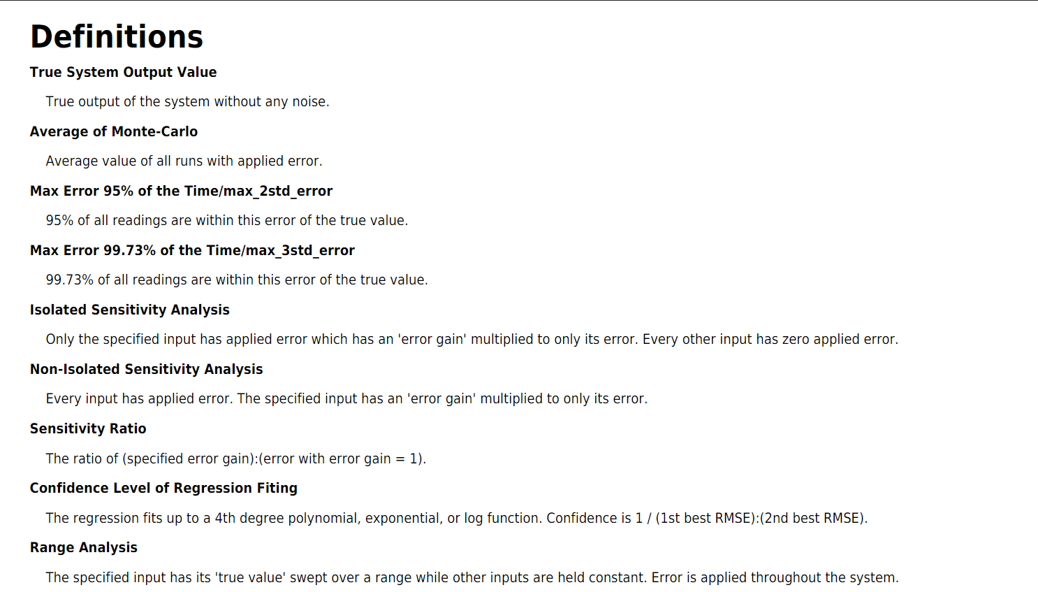
Standard Definitions
The report includes the standard definitions pictured here.
System Setup
There is then a page dedicated for the system that the report was generated for. It begins with the System Governing equation.

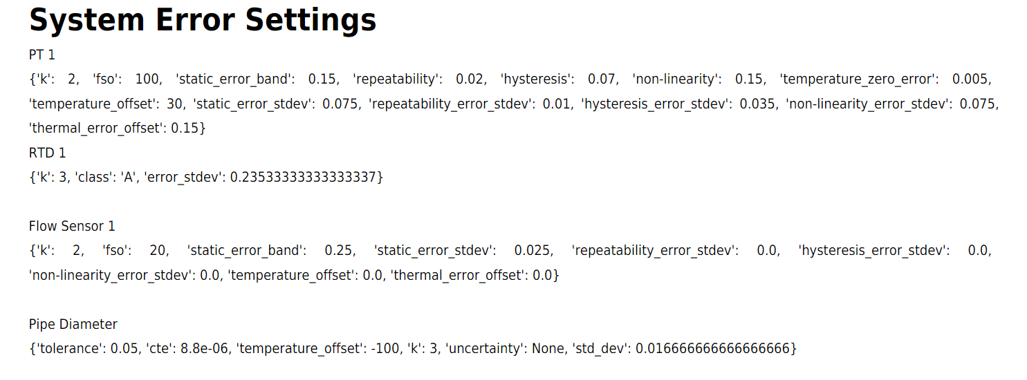
There is then a list of the errors used for each sensor.
System Results
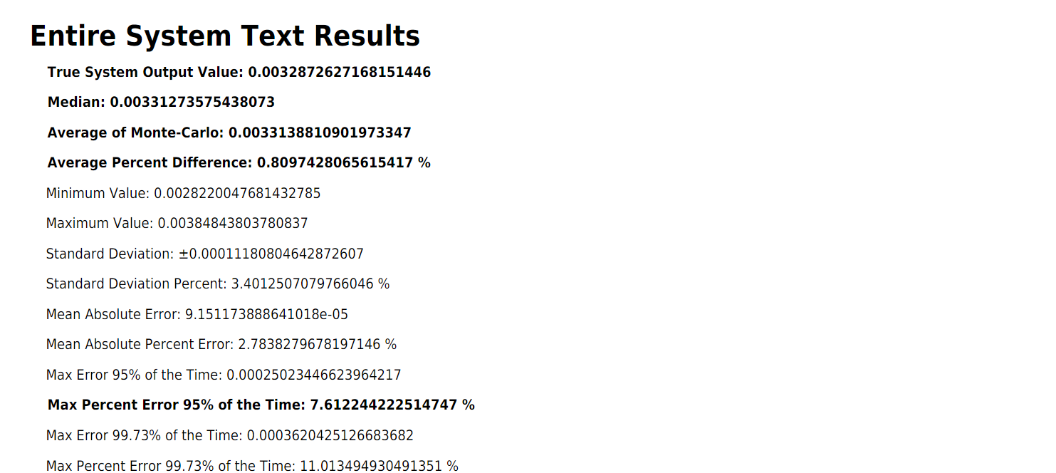
Getting into the Monte Carlo results, the overall system has various numerical results that are shown in text.
There are then two sets of figures. The first figures are histograms, with and without outliers. Immediately next are two scatter plots, again, one with outliers and the other without.
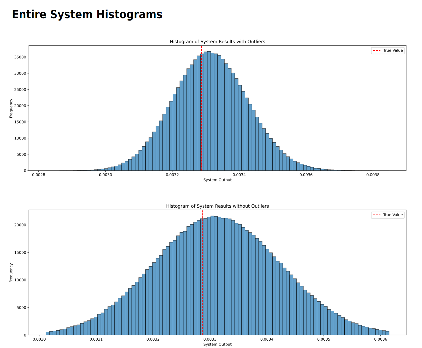
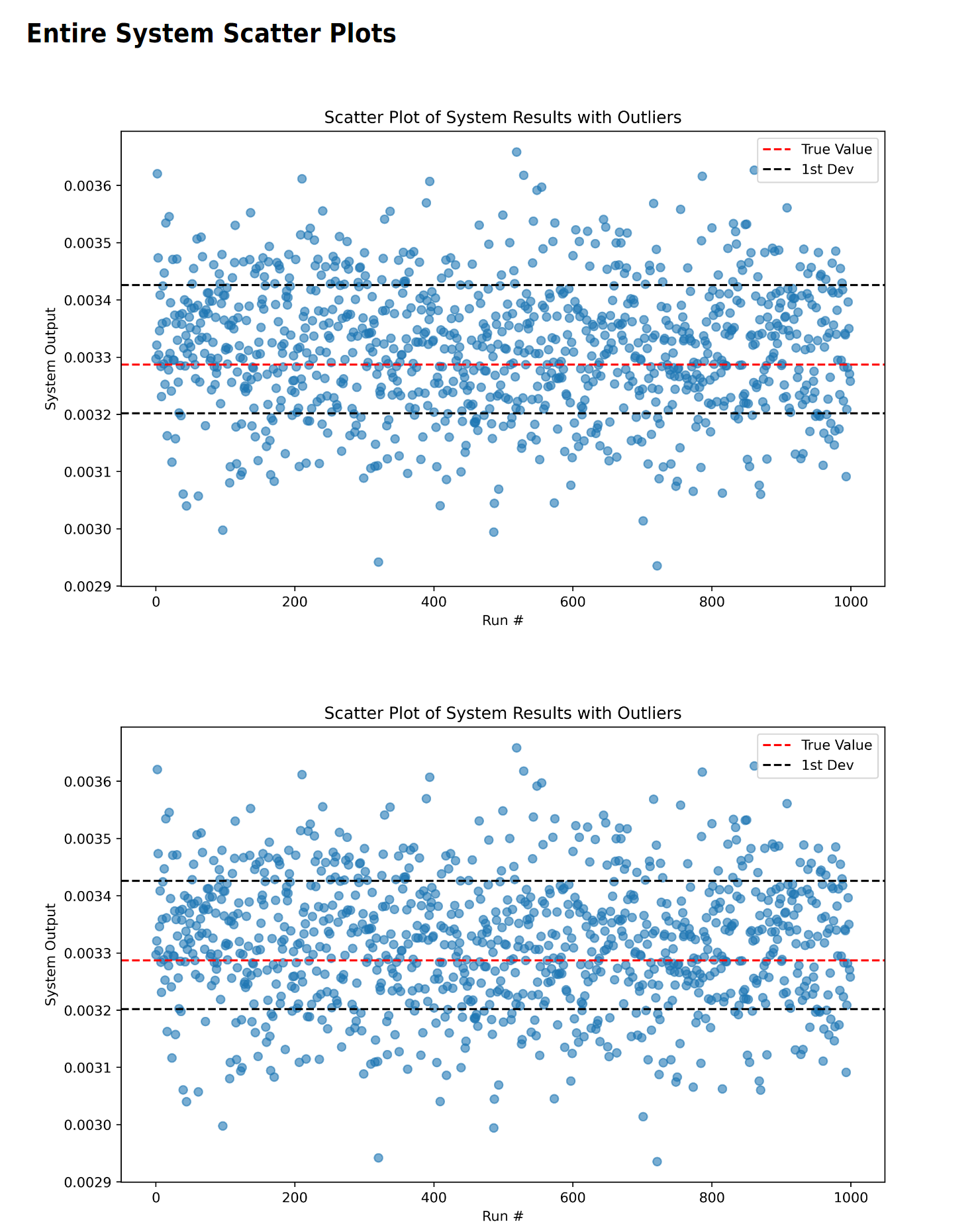
Here we can see the first real results, where the sensor system over estimates the true output due to the various thermal affects that do not average out.
Sensitivity Analysis
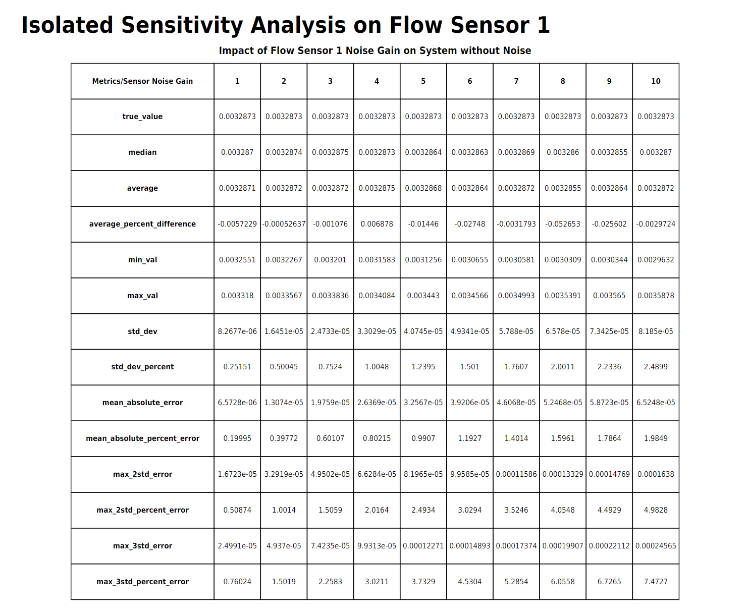
If there is no sensitivity analysis or range analysis desired, this is the end of the report. For each sensor with sensitivity analysis, there will be a table of numerical values followed by two plots looking at how the "error gain" applied to the specific sensor under analysis affects the second standard deviation error of the system. This first table and set of plots is with the sensor "isolated", meaning every other sensor in the system has zero error.
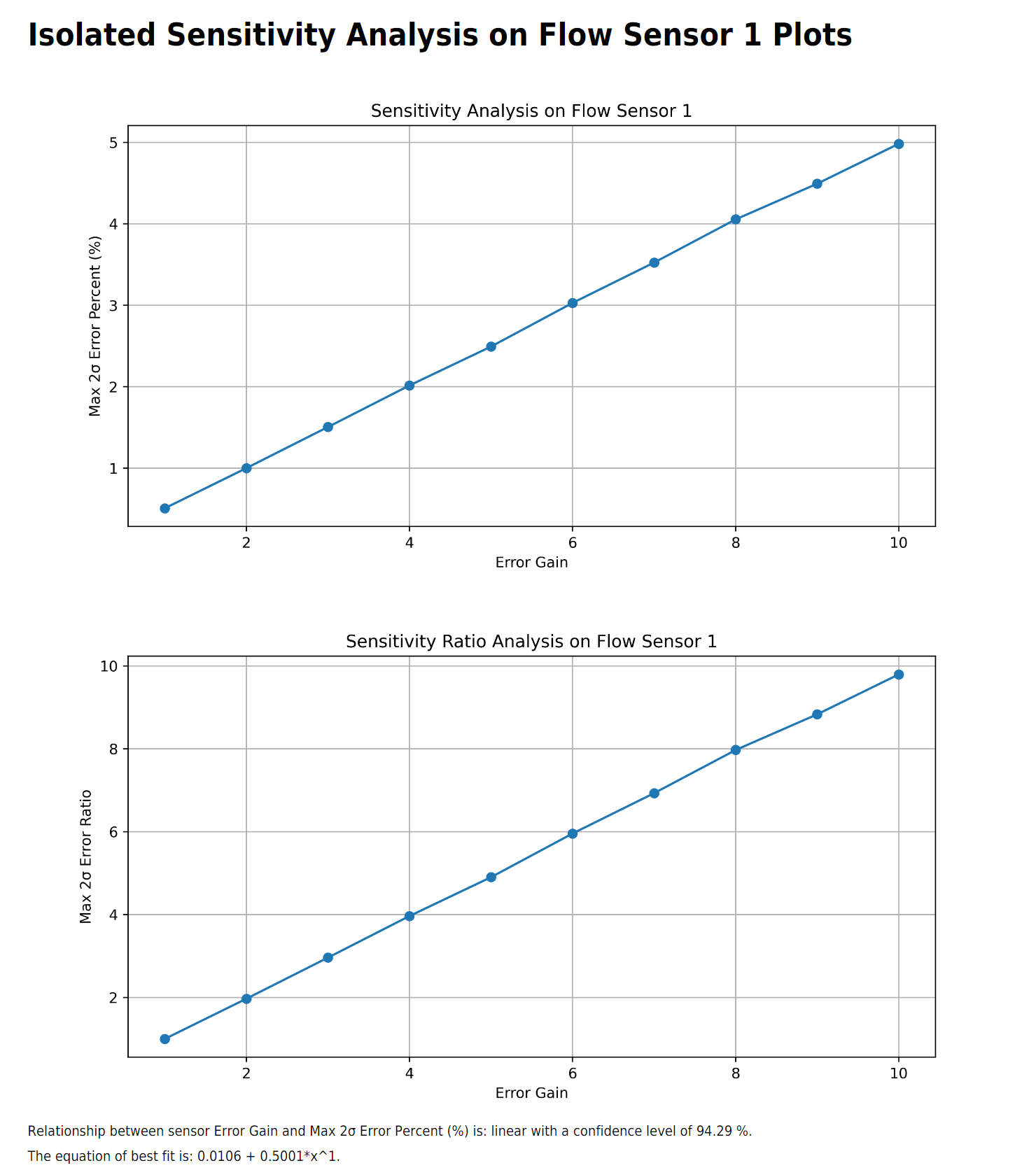
The simulation does its best to rpedict the relationship between entire system error and the "error gain" on the specific sensor.
Continuing with sensitivity analysis, the next table and sets of plots are "non-isolated", meaning the rest of the sensors will have their standard error applied while the sensor under analysis has an "error gain" applied to its base error.
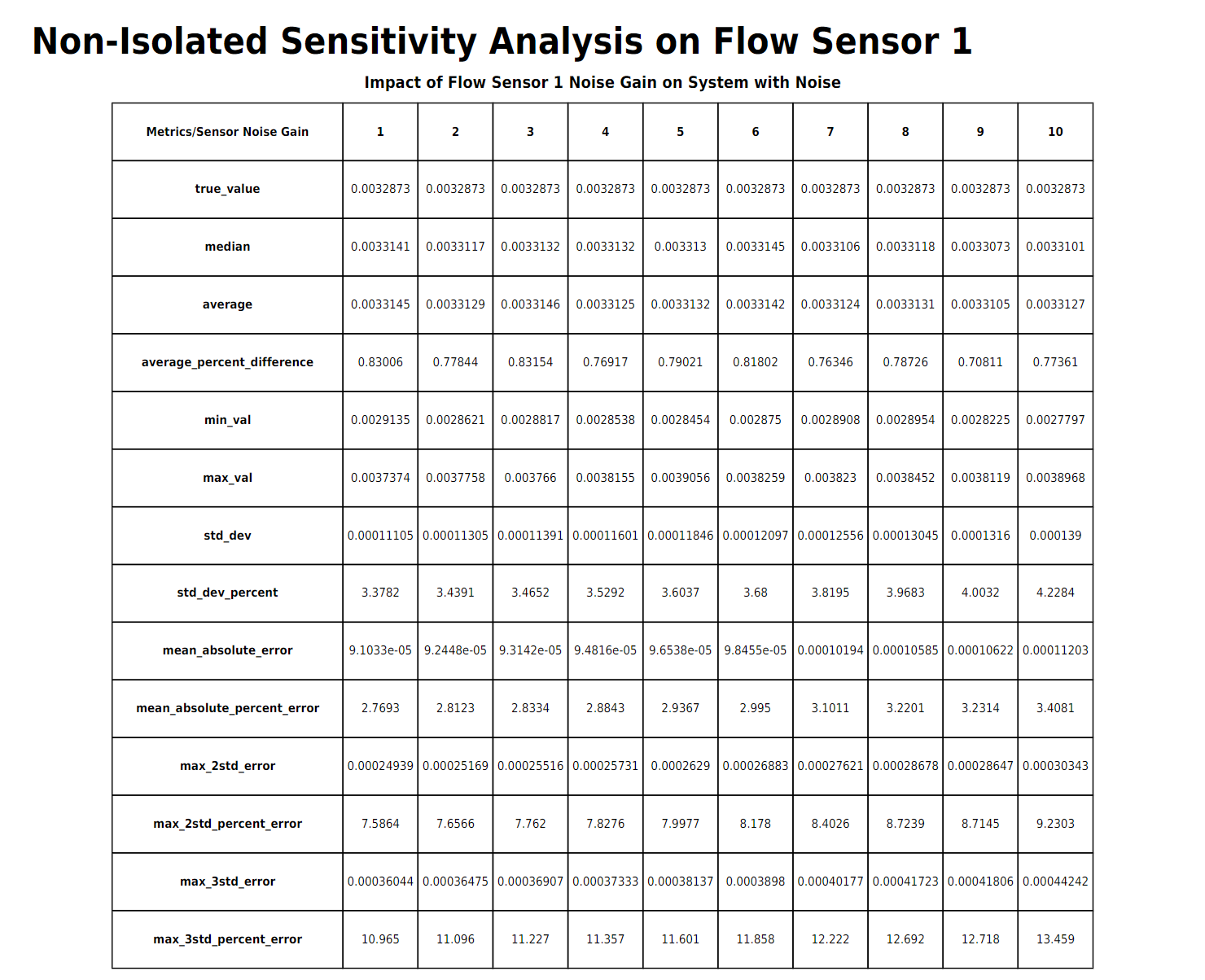
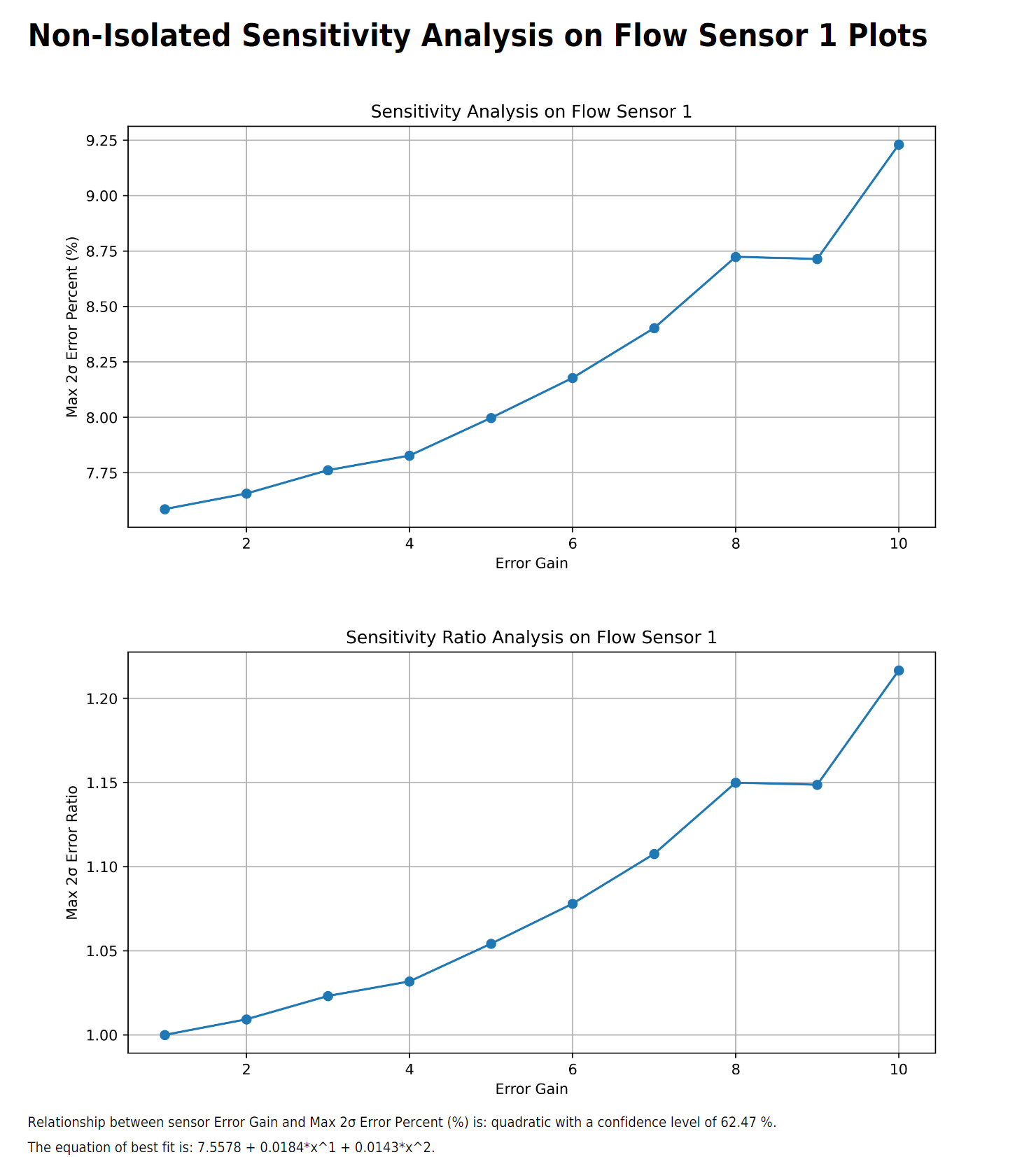
Comparing between isolated and non-isolated sensitivity analysis shows that the flow sensor has minimal impact to the entire system error due to the relatively higher error threshold of the other sensors.
Range Analysis
Similar to sensitivity analysis, range analysis is optional. For each sensor that undergoes range analysis, there is only one plot. This plot sweeps over the possible values that the sensor could have read, giving the user an idea of the error as a function of that sensor's reading. This is primarily impactful for the DensityLookup function.
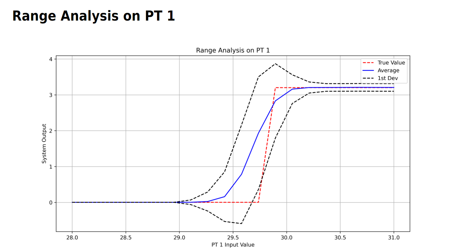
Through range analysis, it is possible to see how small differences in pressure measurement could result in large variations in reported vlue. In this case, the DensityLookup has the fluid changing from a gas to a liquid, where the two-phase mixture has large variations in density and therefore flow rate.